Gaussian derivatives applied to Smemo’s data
Lei Sun
2017-06-17
Last updated: 2018-10-05
workflowr checks: (Click a bullet for more information)-
✔ R Markdown file: up-to-date
Great! Since the R Markdown file has been committed to the Git repository, you know the exact version of the code that produced these results.
-
✔ Environment: empty
Great job! The global environment was empty. Objects defined in the global environment can affect the analysis in your R Markdown file in unknown ways. For reproduciblity it’s best to always run the code in an empty environment.
-
✔ Seed:
set.seed(12345)The command
set.seed(12345)was run prior to running the code in the R Markdown file. Setting a seed ensures that any results that rely on randomness, e.g. subsampling or permutations, are reproducible. -
✔ Session information: recorded
Great job! Recording the operating system, R version, and package versions is critical for reproducibility.
-
Great! You are using Git for version control. Tracking code development and connecting the code version to the results is critical for reproducibility. The version displayed above was the version of the Git repository at the time these results were generated.✔ Repository version: dce4d3b
Note that you need to be careful to ensure that all relevant files for the analysis have been committed to Git prior to generating the results (you can usewflow_publishorwflow_git_commit). workflowr only checks the R Markdown file, but you know if there are other scripts or data files that it depends on. Below is the status of the Git repository when the results were generated:
Note that any generated files, e.g. HTML, png, CSS, etc., are not included in this status report because it is ok for generated content to have uncommitted changes.Ignored files: Ignored: .DS_Store Ignored: .Rhistory Ignored: .Rproj.user/ Ignored: analysis/.DS_Store Ignored: analysis/BH_robustness_cache/ Ignored: analysis/FDR_Null_cache/ Ignored: analysis/FDR_null_betahat_cache/ Ignored: analysis/Rmosek_cache/ Ignored: analysis/StepDown_cache/ Ignored: analysis/alternative2_cache/ Ignored: analysis/alternative_cache/ Ignored: analysis/ash_gd_cache/ Ignored: analysis/average_cor_gtex_2_cache/ Ignored: analysis/average_cor_gtex_cache/ Ignored: analysis/brca_cache/ Ignored: analysis/cash_deconv_cache/ Ignored: analysis/cash_fdr_1_cache/ Ignored: analysis/cash_fdr_2_cache/ Ignored: analysis/cash_fdr_3_cache/ Ignored: analysis/cash_fdr_4_cache/ Ignored: analysis/cash_fdr_5_cache/ Ignored: analysis/cash_fdr_6_cache/ Ignored: analysis/cash_paper_fig_leukemia_cache/ Ignored: analysis/cash_plots_2_cache/ Ignored: analysis/cash_plots_3_cache/ Ignored: analysis/cash_plots_cache/ Ignored: analysis/cash_sim_1_cache/ Ignored: analysis/cash_sim_2_cache/ Ignored: analysis/cash_sim_3_cache/ Ignored: analysis/cash_sim_4_cache/ Ignored: analysis/cash_sim_5_cache/ Ignored: analysis/cash_sim_6_cache/ Ignored: analysis/cash_sim_7_cache/ Ignored: analysis/correlated_z_2_cache/ Ignored: analysis/correlated_z_3_cache/ Ignored: analysis/correlated_z_cache/ Ignored: analysis/create_null_cache/ Ignored: analysis/cutoff_null_cache/ Ignored: analysis/design_matrix_2_cache/ Ignored: analysis/design_matrix_cache/ Ignored: analysis/diagnostic_ash_cache/ Ignored: analysis/diagnostic_correlated_z_2_cache/ Ignored: analysis/diagnostic_correlated_z_3_cache/ Ignored: analysis/diagnostic_correlated_z_cache/ Ignored: analysis/diagnostic_plot_2_cache/ Ignored: analysis/diagnostic_plot_cache/ Ignored: analysis/efron_leukemia_cache/ Ignored: analysis/fitting_normal_cache/ Ignored: analysis/gaussian_derivatives_2_cache/ Ignored: analysis/gaussian_derivatives_3_cache/ Ignored: analysis/gaussian_derivatives_4_cache/ Ignored: analysis/gaussian_derivatives_5_cache/ Ignored: analysis/gaussian_derivatives_cache/ Ignored: analysis/gd-ash_cache/ Ignored: analysis/gd_delta_cache/ Ignored: analysis/gd_lik_2_cache/ Ignored: analysis/gd_lik_cache/ Ignored: analysis/gd_w_cache/ Ignored: analysis/knockoff_10_cache/ Ignored: analysis/knockoff_2_cache/ Ignored: analysis/knockoff_3_cache/ Ignored: analysis/knockoff_4_cache/ Ignored: analysis/knockoff_5_cache/ Ignored: analysis/knockoff_6_cache/ Ignored: analysis/knockoff_7_cache/ Ignored: analysis/knockoff_8_cache/ Ignored: analysis/knockoff_9_cache/ Ignored: analysis/knockoff_cache/ Ignored: analysis/knockoff_var_cache/ Ignored: analysis/marginal_z_alternative_cache/ Ignored: analysis/marginal_z_cache/ Ignored: analysis/mosek_reg_2_cache/ Ignored: analysis/mosek_reg_4_cache/ Ignored: analysis/mosek_reg_5_cache/ Ignored: analysis/mosek_reg_6_cache/ Ignored: analysis/mosek_reg_cache/ Ignored: analysis/pihat0_null_cache/ Ignored: analysis/plot_diagnostic_cache/ Ignored: analysis/poster_obayes17_cache/ Ignored: analysis/real_data_simulation_2_cache/ Ignored: analysis/real_data_simulation_3_cache/ Ignored: analysis/real_data_simulation_4_cache/ Ignored: analysis/real_data_simulation_5_cache/ Ignored: analysis/real_data_simulation_cache/ Ignored: analysis/rmosek_primal_dual_2_cache/ Ignored: analysis/rmosek_primal_dual_cache/ Ignored: analysis/seqgendiff_cache/ Ignored: analysis/simulated_correlated_null_2_cache/ Ignored: analysis/simulated_correlated_null_3_cache/ Ignored: analysis/simulated_correlated_null_cache/ Ignored: analysis/simulation_real_se_2_cache/ Ignored: analysis/simulation_real_se_cache/ Ignored: analysis/smemo_2_cache/ Ignored: data/LSI/ Ignored: docs/.DS_Store Ignored: docs/figure/.DS_Store Ignored: output/fig/
Expand here to see past versions:
| File | Version | Author | Date | Message |
|---|---|---|---|---|
| rmd | dce4d3b | Lei Sun | 2018-10-05 | smemo |
| html | 07bc761 | LSun | 2018-09-05 | Build site. |
| rmd | 653748b | LSun | 2018-09-05 | wflow_publish(“analysis/smemo_2.rmd”) |
| html | 4d653b1 | LSun | 2018-05-15 | Build site. |
| html | 140be7f | LSun | 2018-05-12 | Build site. |
| rmd | 0720bc6 | LSun | 2018-05-12 | Update to 1.0 |
| html | 0720bc6 | LSun | 2018-05-12 | Update to 1.0 |
| rmd | cc0ab83 | Lei Sun | 2018-05-11 | update |
| html | 0f36d99 | LSun | 2017-12-21 | Build site. |
| html | 853a484 | LSun | 2017-11-07 | Build site. |
| html | 1ea081a | LSun | 2017-07-03 | sites |
| html | 86fd092 | LSun | 2017-06-18 | mouse hearts |
| rmd | 7e779ed | LSun | 2017-06-18 | smemo |
| rmd | 8ecbed7 | LSun | 2017-06-18 | mouse hearts |
| rmd | f2fdaf0 | LSun | 2017-06-18 | smemo |
| html | f2fdaf0 | LSun | 2017-06-18 | smemo |
Introduction
Re-analyze Smemo et al 2014’s mouse heart RNA-seq data after discussion with Matthew.
counts.mat = read.table("../data/smemo.txt", header = T, row.name = 1)
counts.mat = counts.mat[, -5]
Gene selection
Only use genes with total counts of \(4\) samples \(\geq 5\).
counts = counts.mat[rowSums(counts.mat) >= 5, ]
design = model.matrix(~c(0, 0, 1, 1))
Number of selected genes: 17191Summary statistics
source("../code/count_to_summary.R")
summary <- count_to_summary(counts, design)
betahat <- summary$betahat
sebetahat <- summary$sebetahat
z <- summary$z
Fitting \(z\) with Gaussian derivatives
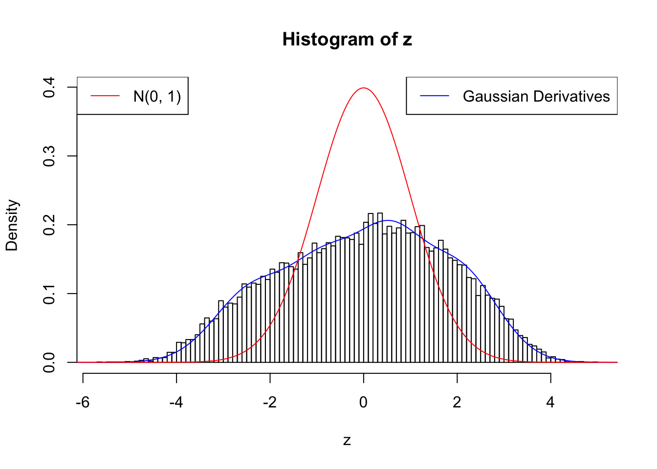
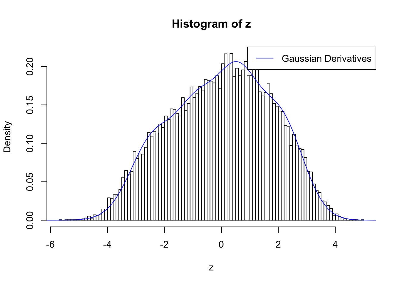
With stretch GD can fit \(z\) scores, but it seems there should be signals.
GD Coefficients:0 : 1 ; 1 : 9.38194912994929e-05 ; 2 : 1.5379335123459 ; 3 : 0.292831264364913 ; 4 : 1.43125454770929 ; 5 : 0.470871356054445 ; 6 : 0.541466442665842 ; 7 : 0.277227258172747 ; 8 : -9.35856044783229e-07 ; 9 : 0.0205987809594603 ; 10 : -3.85399012090005e-08 ;
Expand here to see past versions of fitting gaussian derivatives-1.png:
| Version | Author | Date |
|---|---|---|
| 140be7f | LSun | 2018-05-12 |
| 0f36d99 | LSun | 2017-12-21 |
| f2fdaf0 | LSun | 2017-06-18 |

Discovered by BH and ASH
Feeding summary statistics to BH and ASH, both give thousands of discoveries.
fit.BH = p.adjust((1 - pnorm(abs(z))) * 2, method = "BH")
## Number of discoveries by BH
sum(fit.BH <= 0.05)
[1] 2541fit.ash = ashr::ash(betahat, sebetahat, method = "fdr")
## Number of discoveries by ASH
sum(get_svalue(fit.ash) <= 0.05)[1] 6440Fitting ASH first or Gaussian derivatives first
Using default setting \(L = 10\), \(\lambda = 10\), \(\rho = 0.5\), compare the GD-ASH results by fitting ASH first vs fitting GD first. They indeed arrive at different local minima.
fit.gdash.ASH <- gdash(betahat, sebetahat,
                       gd.priority = FALSE)
## Regularized log-likelihood by fitting ASH first
fit.gdash.ASH$loglik
[1] -12483.86fit.gdash.GD <- gdash(betahat, sebetahat)
## Regularized log-likelihood by fitting GD first
fit.gdash.GD$loglik[1] -22136.92GD-ASH with larger penalties on \(w\)
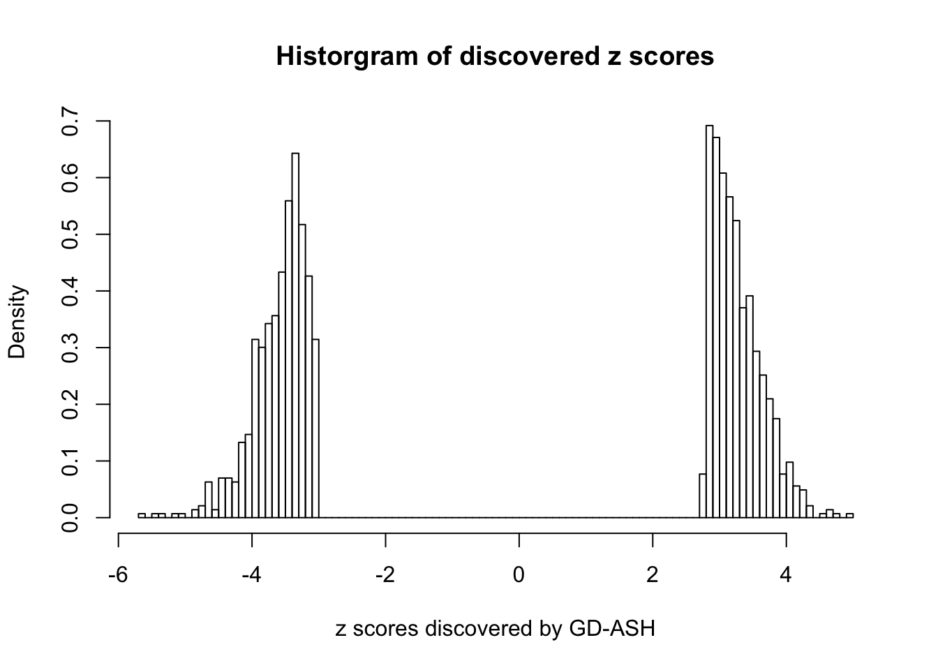
Using \(\lambda = 50\), \(\rho = 0.1\), fitting ASH first and GD first give the same result, and produce 1400+ discoveries with \(q\) values \(\leq 0.05\), all of which are discovered by BH.
L = 10
lambda = 50
rho = 0.1
fit.gdash.ASH <- gdash(betahat, sebetahat,
                       gd.ord = L, w.lambda = lambda, w.rho = rho,
                       gd.priority = FALSE)
## Regularized log-likelihood by fitting ASH first
fit.gdash.ASH$loglik
[1] -13651.59## Number of discoveries
sum(fit.gdash.ASH$qvalue <= 0.05)[1] 1431fit.gdash.GD <- gdash(betahat, sebetahat,
gd.ord = L, w.lambda = lambda, w.rho = rho,
gd.priority = TRUE)
## Regularized log-likelihood by fitting GD first
fit.gdash.GD$loglik[1] -13651.59## Number of discoveries
sum(fit.gdash.GD$qvalue <= 0.05)[1] 1431GD Coefficients:0 : 1 ; 1 : -0.0475544308510135 ; 2 : 0.707888470469342 ; 3 : 0.149489828947119 ; 4 : -8.97499076623316e-14 ; 5 : 0.109281416075664 ; 6 : -3.00530934822662e-13 ; 7 : 0.0783545592042359 ; 8 : -2.99572304462426e-13 ; 9 : 0.0911488252640105 ; 10 : -2.99578347875936e-13 ;
Fitting CASH
source("../code/gdash_lik.R")
source("../code/gdfit.R")
library(edgeR)
Loading required package: limmalibrary(limma)
library(locfdr)counts.mat = read.table("../data/smemo.txt", header = T, row.name = 1)
counts.mat = counts.mat[, -5]
counts = counts.mat[rowSums(counts.mat) >= 5, ]
design = model.matrix(~c(0, 0, 1, 1))
dgecounts = edgeR::calcNormFactors(edgeR::DGEList(counts = counts, group = design[, 2]))
v = limma::voom(dgecounts, design, plot = FALSE)
lim = limma::lmFit(v)
r.ebayes = limma::eBayes(lim)
p = r.ebayes$p.value[, 2]
t = r.ebayes$t[, 2]
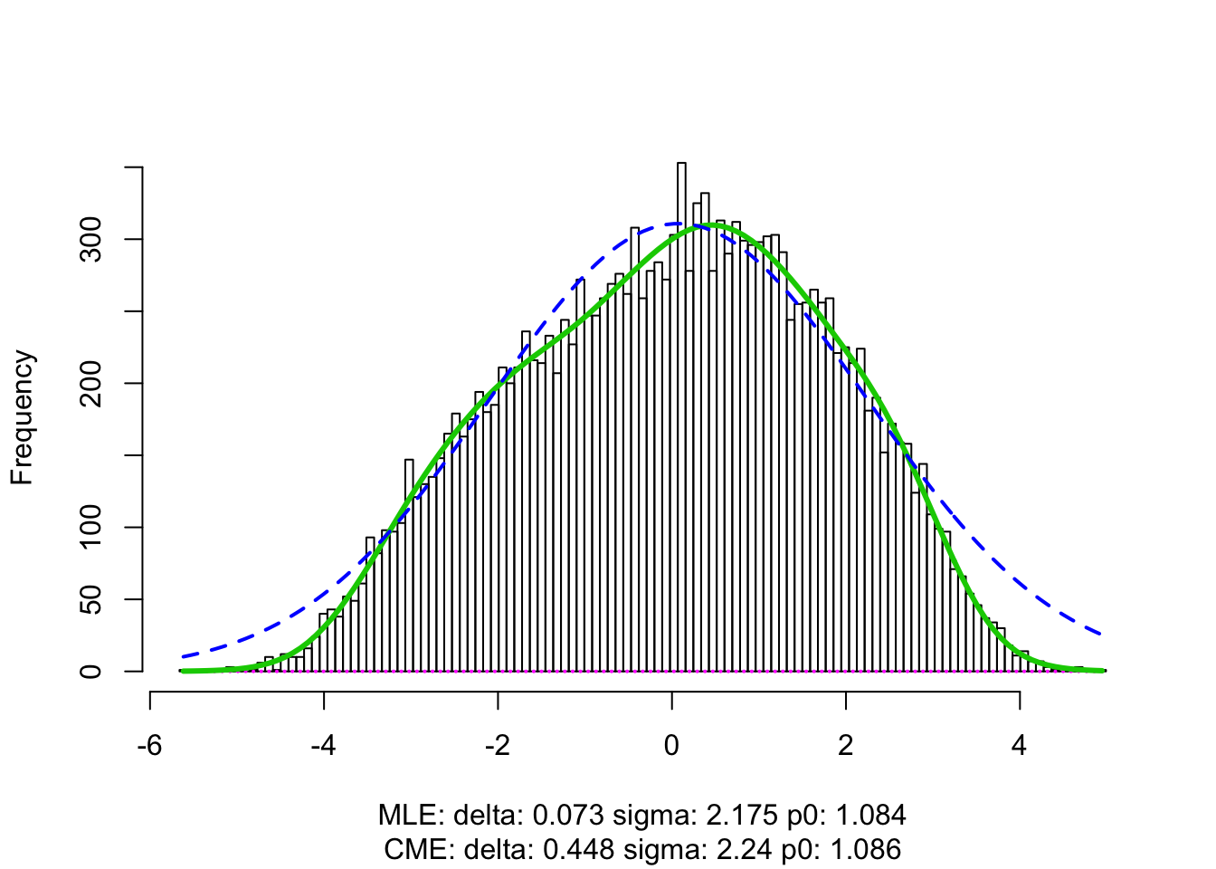
z = -sign(t) * qnorm(p/2)fit.locfdr <- locfdr(z)
Expand here to see past versions of analysis-1.png:
| Version | Author | Date |
|---|---|---|
| 07bc761 | LSun | 2018-09-05 |
fit.qvalue <- qvalue::qvalue(p)betahat = lim$coefficients[, 2]
sebetahat = betahat / z
fit.cash <- gdash(betahat, sebetahat, gd.ord = 10)
fit.ash <- ashr::ash(betahat, sebetahat, mixcompdist = "normal", method = "fdr")x.plot <- seq(-10, 10, length = 1000)
gd.ord <- 10
hermite = Hermite(gd.ord)
gd0.std = dnorm(x.plot)
matrix_lik_plot = cbind(gd0.std)
for (i in 1 : gd.ord) {
gd.std = (-1)^i * hermite[[i]](x.plot) * gd0.std / sqrt(factorial(i))
matrix_lik_plot = cbind(matrix_lik_plot, gd.std)
}
y.plot = matrix_lik_plot %*% fit.cash$w * fit.cash$fitted_g$pi[1]
method.col <- scales::hue_pal()(5)
# method.col <- c("#377eb8", "#984ea3", "#4daf4a", "#ff7f00", "#e41a1c")
setEPS()
postscript("../output/fig/mouseheart.eps", height = 5, width = 12)
par(mfrow = c(1, 2))
hist(z, prob = TRUE, main = "", xlab = expression(paste(z, "-scores")), cex.lab = 1.25)
lines(x.plot, y.plot, col = method.col[5], lwd = 2)
lines(x.plot, dnorm(x.plot), col =
"orange"
# method.col[2]
, lty = 2, lwd = 2)
lines(x.plot, dnorm(x.plot, fit.locfdr$fp0[3, 1], fit.locfdr$fp0[3, 2]) * fit.locfdr$fp0[3, 3], col = method.col[3], lty = 2, lwd = 2)
legend("topleft", col = c("orange", method.col[3], method.col[5]), lty = c(2, 2, 1), legend = c("N(0, 1)", "Empirical null", expression(pi[0]~hat(f))), bty = "n", cex = 1.25)
par(mar = par("mar") + c(0, 1, 0, 0))
g1 <- fit.cash$fitted_g
g1.plot.x <- seq(-0.5, 0.5, length = 1000)
g1.plot.y <- rowSums(sapply(2 : length(g1$pi), function (i) {g1$pi[i] * dnorm(g1.plot.x, g1$mean[i], g1$sd[i])}))
plot(g1.plot.x, g1.plot.y, xlim = c(-0.35, 0.35), type = "l", xlab = expression(paste(theta, " (", log[2], " fold change)")), ylab = expression(hat(g)[1](theta)), cex.lab = 1.25)
dev.off()quartz_off_screen
2 Session information
sessionInfo()R version 3.4.3 (2017-11-30)
Platform: x86_64-apple-darwin15.6.0 (64-bit)
Running under: macOS High Sierra 10.13.6
Matrix products: default
BLAS: /Library/Frameworks/R.framework/Versions/3.4/Resources/lib/libRblas.0.dylib
LAPACK: /Library/Frameworks/R.framework/Versions/3.4/Resources/lib/libRlapack.dylib
locale:
[1] en_US.UTF-8/en_US.UTF-8/en_US.UTF-8/C/en_US.UTF-8/en_US.UTF-8
attached base packages:
[1] stats graphics grDevices utils datasets methods base
other attached packages:
[1] locfdr_1.1-8 edgeR_3.20.9 limma_3.34.9
[4] ashr_2.2-7 Rmosek_8.0.69 PolynomF_1.0-2
[7] CVXR_0.95 REBayes_1.3 Matrix_1.2-14
[10] SQUAREM_2017.10-1 EQL_1.0-0 ttutils_1.0-1
loaded via a namespace (and not attached):
[1] qvalue_2.10.0 locfit_1.5-9.1 reshape2_1.4.3
[4] splines_3.4.3 lattice_0.20-35 colorspace_1.3-2
[7] htmltools_0.3.6 yaml_2.1.19 gmp_0.5-13.1
[10] rlang_0.2.0 R.oo_1.22.0 pillar_1.2.2
[13] Rmpfr_0.7-0 R.utils_2.6.0 bit64_0.9-7
[16] scs_1.1-1 foreach_1.4.4 plyr_1.8.4
[19] stringr_1.3.1 munsell_0.4.3 gtable_0.2.0
[22] workflowr_1.1.1 R.methodsS3_1.7.1 codetools_0.2-15
[25] evaluate_0.10.1 knitr_1.20 doParallel_1.0.11
[28] pscl_1.5.2 parallel_3.4.3 Rcpp_0.12.16
[31] backports_1.1.2 scales_0.5.0 truncnorm_1.0-8
[34] bit_1.1-13 ggplot2_2.2.1 digest_0.6.15
[37] stringi_1.2.2 grid_3.4.3 rprojroot_1.3-2
[40] ECOSolveR_0.4 tools_3.4.3 magrittr_1.5
[43] lazyeval_0.2.1 tibble_1.4.2 whisker_0.3-2
[46] MASS_7.3-50 assertthat_0.2.0 rmarkdown_1.9
[49] iterators_1.0.9 R6_2.2.2 git2r_0.21.0
[52] compiler_3.4.3 This reproducible R Markdown analysis was created with workflowr 1.1.1